Examples
In the following we provide some examples that demonstrate the use of
potentials, the background equations, computation of the comoving Hubble
horizon, the slow-roll approximation of the primordial power spectrum, and
finally the fully numeric primordial power spectrum making use of the
pyoscode package to solve the oscillatory ODE.
Importing routines used for all examples:
import numpy as np
import matplotlib.pyplot as plt

from primpy.parameters import K_STAR
import primpy.potentials as pp
from primpy.events import UntilNEvent, InflationEvent, CollapseEvent
from primpy.initialconditions import InflationStartIC, ISIC_Nt
from primpy.time.inflation import InflationEquationsT as InflationEquations
from primpy.solver import solve
from primpy.oscode_solver import solve_oscode
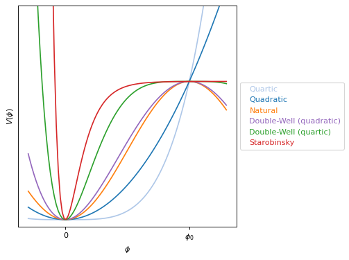
Potentials
There are various large, single, scalar field inflation models implemented in
primpy.potentials. The following plot gives an overview:
phi_range = np.linspace(-3, 13, 100)

mn2 = pp.QuadraticPotential(Lambda=1/10**(1/2))
mn4 = pp.QuarticPotential(Lambda=1/10)
nat = pp.NaturalPotential(Lambda=1, phi0=10)
dw2 = pp.DoubleWell2Potential(Lambda=1, phi0=10)
dw4 = pp.DoubleWell4Potential(Lambda=1, phi0=10)
stb = pp.StarobinskyPotential(Lambda=1)

fig, ax = plt.subplots()
ax.plot(phi_range, mn4.V(phi=phi_range), c=plt.cm.tab20(1), label="Quartic")
ax.plot(phi_range, mn2.V(phi=phi_range), c=plt.cm.tab20(0), label="Quadratic")
ax.plot(phi_range, nat.V(phi=phi_range), c=plt.cm.tab20(2), label=nat.tex)
ax.plot(phi_range, dw2.V(phi=phi_range), c=plt.cm.tab20(8), label=dw2.tex)
ax.plot(phi_range, dw4.V(phi=phi_range), c=plt.cm.tab20(4), label=dw4.tex)
ax.plot(phi_range, stb.V(phi=phi_range), c=plt.cm.tab20(6), label=stb.tex)
ax.set_ylim(-0.05, 1.55)
ax.set_yticks([])
ax.set_xticks([0, 10])
ax.set_xticklabels([0, "$\\phi_0$"])
ax.set_xlabel(r"$\phi$")
ax.set_ylabel(r"$V(\phi)$")
ax.legend(bbox_to_anchor=(1, 0.5), loc='center left', labelcolor='linecolor',
          handlelength=0, markerscale=0)
fig.tight_layout()
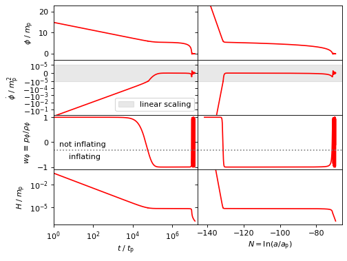
Background equations
Setup: Let’s compute the inflationary background equations in flat space (K=0) for the Starobinsky potential with the following additional parameter setup:
t_eval = np.logspace(5, 8, 2000)
K = 0            # flat universe
N_star = 50      # number of e-folds of inflation after horizon crossing
N_tot = 60       # total number of e-folds of inflation
N_end = 70       # end time/size after inflation, arbitrary in flat universe
delta_N_reh = 2  # extra e-folds after end of inflation to see reheating oscillations
A_s = 2e-9       # amplitude of primordial power spectrum at pivot scale
Pot = pp.StarobinskyPotential
We compute the background equations keeping track of the start and the end of inflation and ending the ODE integration once a given number of e-folds has been reached. We set the initial conditions at the start of inflation and integrate both forwards and backwards in time. We finish by calibrating the scale factor for a flat universe (such that \(a_0=1\)), which comes down to shifting the number of e-folds \(N\) by a constant.
# slow-roll estimate of amplitude `Lambda` and field value `phi_star` at horizon crossing
pot = Pot(A_s=A_s, N_star=N_star, phi_star=None)
phi_guess = pot.sr_N2phi(N=N_tot)
eq = InflationEquations(K=K, potential=pot, track_eta=False)
ev = [UntilNEvent(eq, value=N_end+delta_N_reh),  # decides stopping criterion
      InflationEvent(eq, +1, terminal=False),    # records inflation start
      InflationEvent(eq, -1, terminal=False)]    # records inflation end

# from inflation start forwards in time, optimising to get `N_tot` e-folds of inflation
ic_fore = ISIC_Nt(equations=eq, N_tot=N_tot, N_i=N_end-N_tot, t_i=t_eval[0],
                  phi_i_bracket=[phi_guess-2, phi_guess+2])
fward = solve(ic=ic_fore, events=ev, t_eval=t_eval)
# from inflation start backwards in time
ic_back = InflationStartIC(equations=eq, phi_i=ic_fore.phi_i, N_i=ic_fore.N_i, t_i=t_eval[0],
                           x_end=1)
bward = solve(ic=ic_back, events=ev)
# need to shift time, since we initially did not know the precise starting time of inflation
bward_t = (bward.t - bward.t.min())
fward_t = (fward.t - bward.t.min())
# calibrate the scale factor by providing the number `N_star` of e-folds of inflation after
# horizon crossing of the pivot scale
fward.calibrate_scale_factor(N_star=N_star)
bward.calibrate_scale_factor(N_star=N_star, background=fward)
Plot of some background variables in reduced Planck units. The inflaton field \(\phi\), its first time derivative \(\dot\phi\), the equation-of-state parameter during inflation \(w_\phi\), and the Hubble parameter \(H\):
fig, ax = plt.subplots(4, 2, sharex='col', sharey='row',
                       gridspec_kw={'hspace': 0, 'wspace': 0})

ax[0, 0].set_xlim(1, 2e7)
ax[0, 0].set_ylim(-3, 23)
ax[1, 0].set_ylim(-5e-1, 5e-5)
ax[3, 0].set_ylim(0.5e-7, 1e-0)

ax[0, 0].semilogx(bward_t, bward.phi, c='r')
ax[0, 0].semilogx(fward_t, fward.phi, c='r')
ax[1, 0].semilogx(bward_t, bward.dphidt, c='r')
ax[1, 0].semilogx(fward_t, fward.dphidt, c='r')
ax[1, 0].set_yscale('symlog', linthresh=1e-5)
ax[1, 0].axhspan(-1e-5, 1e-5, color='0.7', alpha=0.3, label="linear scaling")
ax[1, 0].legend()
ax[2, 0].semilogx(bward_t, bward.w, c='r')
ax[2, 0].semilogx(fward_t, fward.w, c='r')
ax[2, 0].axhline(-1/3, ls=':', c='0.5', label=r"$\ddot a=0 \Leftrightarrow V(\phi)=\dot\phi$")
ax[2, 0].text(x=ax[2, 0].get_xlim()[0] * 2, y=-1/3+0.10, s="not inflating", va='bottom')
ax[2, 0].text(x=ax[2, 0].get_xlim()[0] * 2, y=-1/3-0.12, s="    inflating", va='top')
ax[3, 0].loglog(bward_t, bward.H, c='r')
ax[3, 0].loglog(fward_t, fward.H, c='r')

ax[0, 1].plot(bward.N, bward.phi, c='r')
ax[0, 1].plot(fward.N, fward.phi, c='r')
ax[1, 1].plot(bward.N, bward.dphidt, c='r')
ax[1, 1].plot(fward.N, fward.dphidt, c='r')
ax[1, 1].set_yscale('symlog', linthresh=1e-5)
ax[1, 1].axhspan(-1e-5, 1e-5, color='0.7', alpha=0.3, label="linear scaling")
ax[2, 1].plot(fward.N, fward.w, c='r')
ax[2, 1].plot(bward.N, bward.w, c='r')
ax[2, 1].axhline(-1/3, ls=':', c='0.5', label=r"$\ddot a=0 \Leftrightarrow V(\phi)=\dot\phi$")
ax[3, 1].semilogy(bward.N, bward.H, c='r')
ax[3, 1].semilogy(fward.N, fward.H, c='r')

ax[0, 0].set_ylabel(r"$\phi\;/\;m_\mathrm{p}$")
ax[1, 0].set_ylabel(r"$\dot\phi\;/\;m_\mathrm{p}^2$")
ax[2, 0].set_ylabel(r"$w_\phi\,\equiv\,p_\phi/\rho_\phi$")
ax[3, 0].set_ylabel(r"$H\;/\;m_\mathrm{p}$")
ax[3, 0].set_xlabel(r"$t\;/\;t_\mathrm{p}$")
ax[3, 1].set_xlabel(r"$N = \ln(a/a_\mathrm{p})$")

fig.tight_layout()
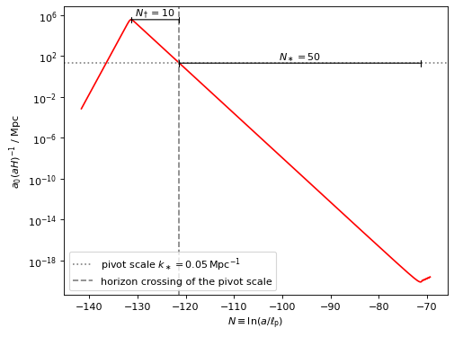
Comoving Hubble horizon
Plot the comoving Hubble horizon which initially increases during kinetic dominance, decreases during inflation, and eventually increases again during reheating:
fig, ax = plt.subplots(1, 1)

ax.semilogy(bward.N, bward.cHH_Mpc, c='r')
ax.semilogy(fward.N, fward.cHH_Mpc, c='r')
ax.set_xlabel(r"$N \equiv \ln(a/\ell_\mathrm{p})$")
ax.set_ylabel(r"$a_0 (aH)^{-1}\ /\ \mathrm{Mpc}$")

ax.axhline(1/K_STAR, ls=':', color='0.5',
           label="pivot scale $k_\\ast=%g\\,\\mathrm{Mpc^{-1}}$" % K_STAR)
ax.axvline(fward.N_cross, ls='--', color='0.5',
           label="horizon crossing of the pivot scale")
ax.text(fward.N_cross+(fward.N_end-fward.N_cross)/2, 1/K_STAR,
        r"$N_\ast=%g$" % fward.N_star, ha='center', va='bottom')
ax.text(fward.N_beg  +(fward.N_cross-fward.N_beg)/2, fward.cHH_Mpc[0],
        r"$N_\dagger=%g$" % (fward.N_tot-fward.N_star), ha='center', va='bottom')
ax.annotate("", xy=(fward.N_cross, 1/K_STAR), xytext=(fward.N_end, 1/K_STAR),
            arrowprops=dict(arrowstyle='|-|', mutation_scale=3, shrinkA=0, shrinkB=0))
ax.annotate("", xy=(fward.N_beg, fward.cHH_Mpc[0]), xytext=(fward.N_cross, fward.cHH_Mpc[0]),
            arrowprops=dict(arrowstyle='|-|', mutation_scale=3, shrinkA=0, shrinkB=0))
ax.legend(loc='lower left')
fig.tight_layout()
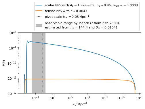
Slow-roll approximation of the primordial power spectrum
Estimate of the distance to recombination to get a sense of the CMB observable range for the primordial power spectrum which depends on the wavenumber \(k\) rather than multipole moment \(\ell\):
r_ast = 144.4
theta_ast = 1.041e-2
D_rec = r_ast / theta_ast
Plot:
fig, ax = plt.subplots(1, 1)
ax.loglog(fward.k_iMpc, fward.P_scalar_approx,
          label=("scalar PPS with " +
                 "$A_\\mathrm{s}\\approx%.3g$, " % fward.A_s +
                 "$n_\\mathrm{s}\\approx%.2g$, " % fward.n_s +
                 "$n_\\mathrm{run}\\approx%.1g$" % fward.n_run))
ax.loglog(fward.k_iMpc, fward.P_tensor_approx,
          label="tensor PPS with $r\\approx%.2g$" % (fward.r))
ax.axvline(K_STAR, ls=':', color='k',
           label="pivot scale $k_\\ast=%g\\,\\mathrm{Mpc^{-1}}$" % K_STAR)
ax.axvspan(2/D_rec, 2500/D_rec, color='0.5', alpha=0.5,
           label="observable range by Planck ($\\ell$ from 2 to 2500), \n" +
                 "estimated from $r_\\ast=%g$ and $\\theta_\\ast=%g$" % (r_ast, theta_ast))
ax.set_ylim(1e-12, 1e-8)
ax.set_ylabel(r"$\mathcal{P}(k)$")
ax.set_xlabel(r"$k\ /\ \mathrm{Mpc^{-1}}$")
ax.legend(bbox_to_anchor=(1, 1), loc='lower right')
fig.tight_layout()
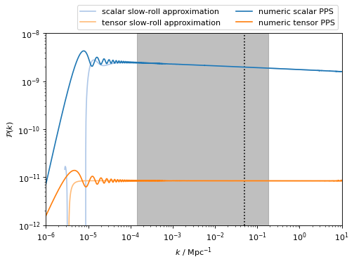
Fully numeric primordial power spectrum
Since we set up a flat universe, there is some arbitrariness in the choice of normalisation of the scale factor \(a_0\) (in curved universes it would have a physical meaning as the radius of the Universe). Hence, there is some extra calibration that needs doing for flat universes:
k_iMpc = np.logspace(-6, 1, 2000)
k_comoving = k_iMpc * fward.a0_Mpc
Compute the primordial power spectrum using pyoscode to solve the
oscillatory ODE.
pps = solve_oscode(background=fward, k=k_comoving, vacuum=('RST',))
fig, ax = plt.subplots(1, 1)
ax.axvline(K_STAR, ls=':', color='k')
ax.axvspan(2/D_rec, 2500/D_rec, color='0.5', alpha=0.5)
ax.loglog(fward.k_iMpc, fward.P_scalar_approx, c=plt.cm.tab20(1),
          label="scalar slow-roll approximation")
ax.loglog(fward.k_iMpc, fward.P_tensor_approx, c=plt.cm.tab20(3),
          label="tensor slow-roll approximation")
ax.loglog(pps.k_iMpc, pps.P_s_RST, c=plt.cm.tab20(0), label="numeric scalar PPS")
ax.loglog(pps.k_iMpc, pps.P_t_RST, c=plt.cm.tab20(2), label="numeric tensor PPS")
ax.set_xlim(pps.k_iMpc[0], pps.k_iMpc[-1])
ax.set_ylim(1e-12, 1e-8)
ax.set_ylabel(r"$\mathcal{P}(k)$")
ax.set_xlabel(r"$k\ /\ \mathrm{Mpc^{-1}}$")
ax.legend(bbox_to_anchor=(1, 1), loc='lower right', ncol=2)
fig.tight_layout()